
Why do we need graphs for image processing?
Image processing over the years has evolved from simple linear averaging filters to highly adaptive non linear filtering operations such as the bilateral filter, moving least squares, BM3D and LARK to name a few. However, a shortcoming of these powerful methods is the lack of interpretability using conventional non-adaptive grid based transform techniques such as Fourier and DCT. In recent years, graphs and the associated spectral decomposition have emerged as a unified representation for image analysis and processing. This area of research is broadly categorized under Graph Signal Processing (GSP), an upcoming field which has heralded several algorithms in various topics (including neural networks - Graph Convolution Networks). Note that with any graph based algorithm, the runtime is generally a function of the number of edges in the graph and so it is often desirable to have a sparse graph which capture the content of the underlying data.
How to represent images using graphs?
In this post, we will focus on the problem of representing images using graphs - What is the right graph to represent images? and is the graph construction method scalable? An image graph is constructed with each pixel as a node with edges between them capturing similarity between the nodes. A standard, naive approach to image graph construction is that of a window based method i.e., each pixel (node) is connected to all neighboring pixels within a window centered at the pixel. These are then weighed using a kernel to quantify similarity. This method is similar to that of the more general K-nearest neighbor (KNN) graph construction where we set K to the window size and choose neighbors based on only spatial distance in image. A problem with this representation is that the sparsity of the image graph formed is entirely dependent on the choice of window size and is not adaptive to the local structure of the image. This poses a problem since this choice is often adhoc with no clear methodology to make the choice as in the case of KNN graphs.
NNK graphs
As an alternative, in our work we leverage the sparse signal approximation perspective of Non Negative Kernel regression (NNK) graphs to the domain of images.
The outline and motivation for NNK graph construction is as follows
- Consider a node i
- Select nodes j with maximum kernel similarity (or equivalently smallest distance)
- These selected nodes can be considered to form a locally adaptive dictionary
- KNN approach corresponds to choosing K maximally correlated atoms in the dictionary formed - a thresholding procedure.
- NNK performs a non negative basis pursuit to identify and obtain an efficient sparse representation.
As a consequence, we observe stable, sparse represetation where the relative position of the underlying data is taken into consideration. This property can be theoretically and geometrically explained using the Kernel Ratio Interval (KRI) as shown in the fig. below. Simply put, given a node j connected to i, NNK looks for additional neighbors that are in different directions i.e., orthogonal.
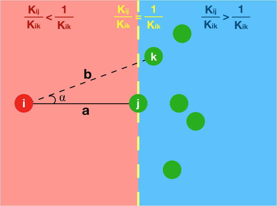
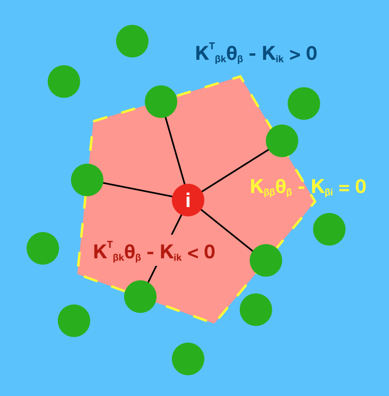
This geometric interpretation along with the pixel position regularity in images and specific characteristics of kernel allows us to learn image graphs in a fast and efficient manner (10x faster than naive NNK).
NNK image graph algorithm
We will use the bilateral filter kernel to construct the image graph, though any kernel that has values in range [0, 1] can be integrated into the NNK image graph framework. As shown in the paper, the bilateral filter with KRI gives us a simple threshold condition (computed offline) on intensity to determine if a pixel k is to be connected given a connected pixel j is connected to the center pixel. We will apply this condition with positive threshold going radially outwards from the center pixel, starting with the four connected neighbors. We confine ourselves to positive thresholds since negative thresholds corresponds to pixels in the opposite side of the pixel window and are less likely to be affected by the connectivity of the current pixel.
The figure below presents the case of NNK image graph algorithm for a 7x7 window centered at pixel i. Note that, conventionally one would connect i to all pixels in the window. In NNK, we start with one of the closest pixel namely j and assume its connected. We observe intensity differences and compare with the precomputed threshold to prune pixels that will not be connected given the connection to j. We perform this step iteratively i.e.,
- Select closest pixel that is not pruned and connect to i
- Apply pruning condition to remove pixels that are below threshold
- Stop when no more pixels are left for processing
Experimental analysis
NNK image graphs have far fewer edges compared to its naive KNN-like counterparts (90% reduction in edges for a 11x11 window). This massive reduction in number of edges speeds up graph filtering operations in images by atleast 15x without loss in representation. Infact, we show that graph processing and transforms based on NNK image graphs are much better in capturing image content and resulting filtering performance.
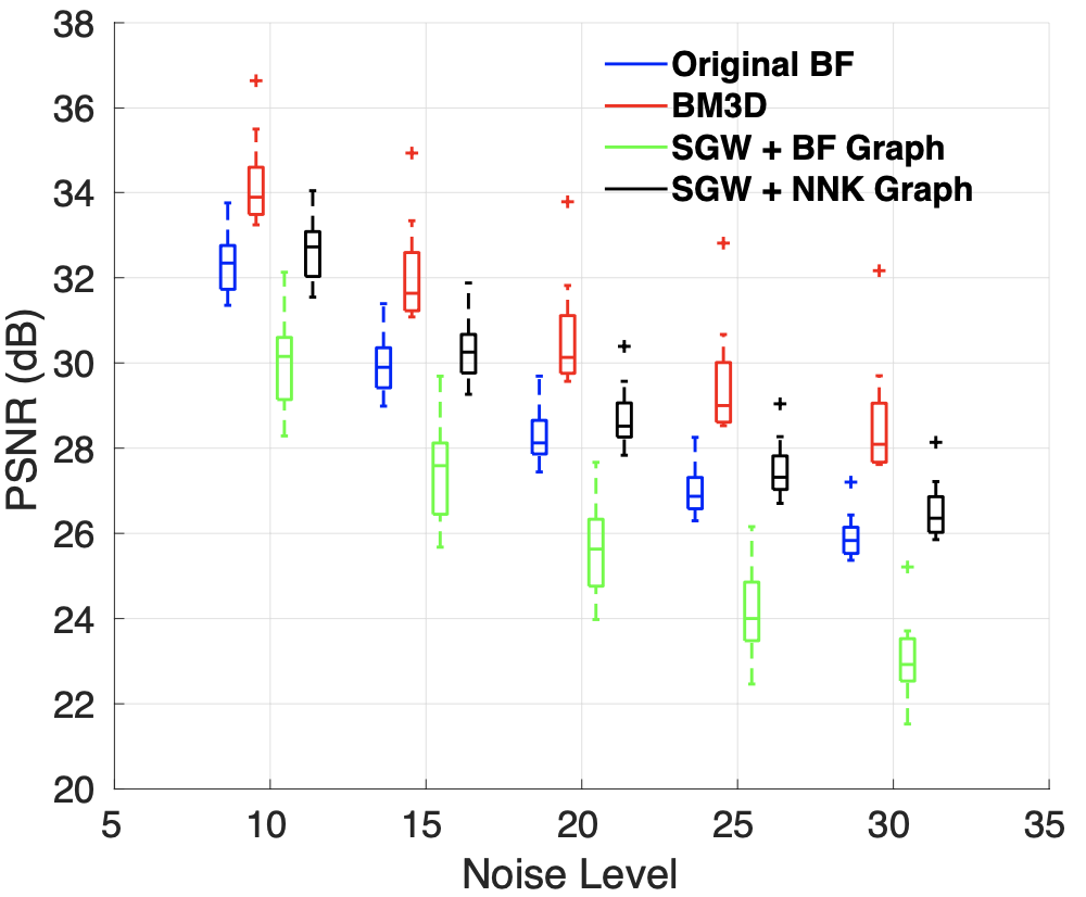
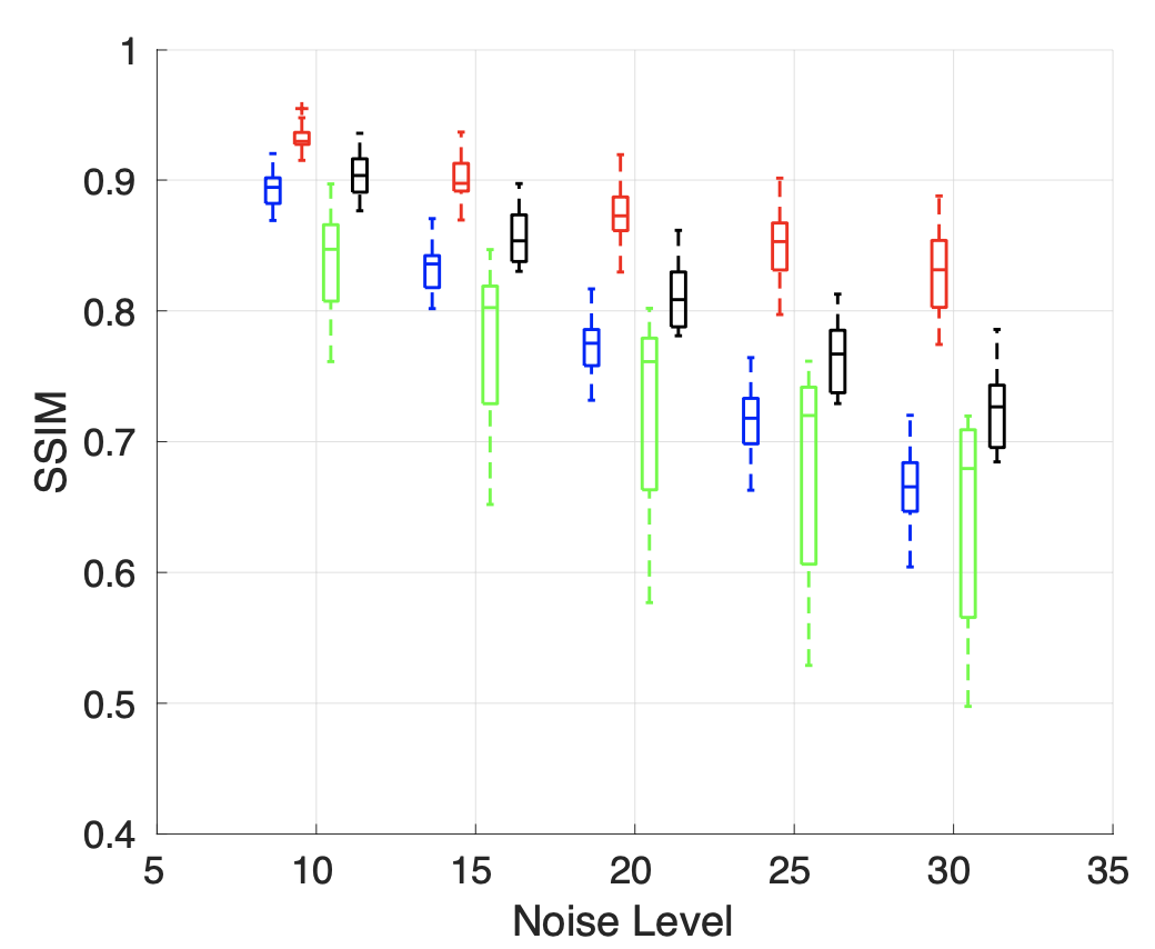
Further, spectral image denoising based on NNK graphs shows promising performance. We observe that unlike BF graph based denoising whose performance worsens compared to its original non-graph based denoiser, NNK image graph based filtering improves performance achieving metrics close to more complex methods such as BM3D.
Future Directions
In this article, we looked at a scalable, efficient graph construction framework for images with interpretable connectivity and robust performance. Further, the local nature of the algorithm allows for parallelized execution. We believe we are only scratching the surface with bilateral filter kernels and that better performance and representation is possible by incorporating more complex kernels such as non local means, BM3D to name a few.
Source code available at github.com/STAC-USC/NNK_Image_graph