Note: This is based on a presentation done at Tenyx

Understanding MLPs Through the Lens of Hashing

When we think about Multi-Layer Perceptrons (MLPs), we often visualize them as interconnected units processing information. However, there’s an elegant alternative perspective: MLPs are

1. locality sensitive hashing functions that partition an input space, and
2. mappings that linearly transform these partitions

This mental model, which I’ll share from my research experiences at Tenyx, provides powerful insights into how neural networks learn and several algorithmic improvements that are applicable to even large language models.

The Basic Building Block: Neurons as Hyperplanes

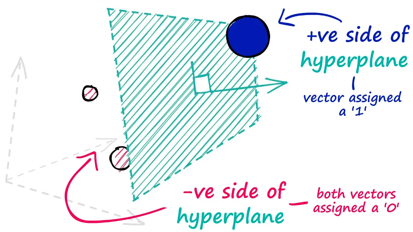
At its core, a single neuron (perceptron) acts as a hyperplane that divides the input space into two regions. When we apply a ReLU activation function, we’re essentially deciding which side of this hyperplane we’re interested in. This simple geometric interpretation leads to a fascinating observation: each neuron creates a partition in the input space. For details about hashing, hyperplanes, and partitions, refer to this blog at Pinecone.

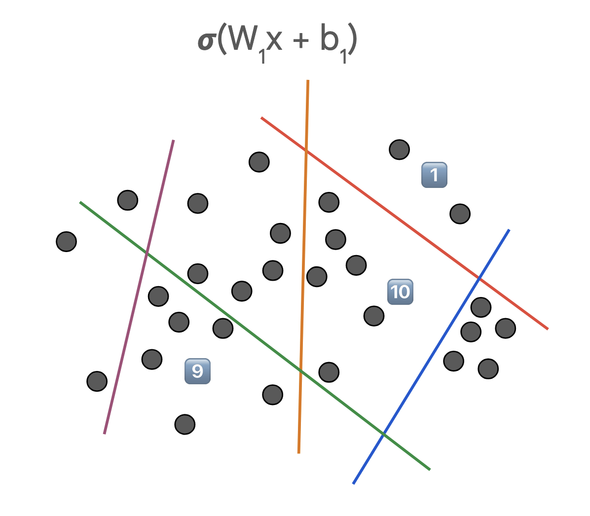
Now, when we stack multiple neurons together to form a 1-layer neural network, something more complex happens. Each neuron creates increasingly complex hashing functions (regions) of the input space. Figure 2 presents an example of such a scenario where each partition leads to a hash code with a mapping function:

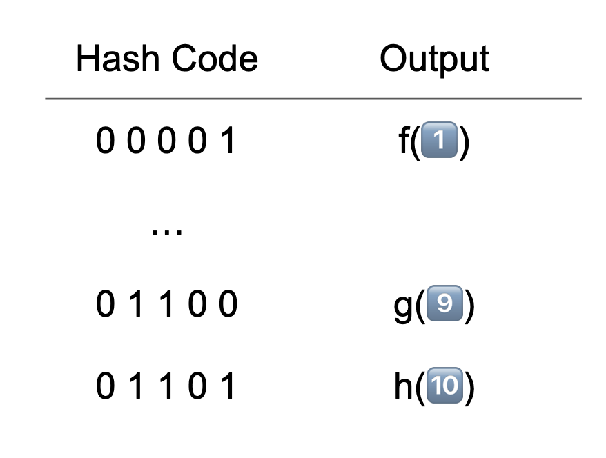
Note how in this example of a single-layer network with 5 neurons, one could theoretically create 2^5 = 32 different partitions. However, in practice, we often find that only a subset of these partitions (in this case, 7) are actually utilized, i.e., contain data. This observation has profound implications for both model efficiency and learning dynamics.

An interesting question arises at this point: How does a wide (more neurons) network differ from a deep (multiple layers) network?

It is clear that having more neurons would lead to more (possibly finer) partitions and can learn any function on the input space. This is often referred to as the Universal Approximation, which essentially means that any function can be represented by a single hidden layer network. However, it has been since established that going deeper has better learning dynamics than a single layer network - think hierarchical refinement of the transformation achieved with a single layer. This partitioning and mapping achieved by ReLU MLPs are equivalent to Continuous Piecewise Affine transforms.

Learning as Partition Refinement

When an MLP learns, it’s essentially doing two things simultaneously:

1. Adjusting the partitions (by rotating and shifting hyperplanes)
2. Modifying the mapping from these partitions to outputs

A nice interactive playground to understand and visualize this is available at Perceptron visualization and MLP visualization. Do check these out to get an intuitive understanding of what you read so far!

The dual nature of learning helps explain why neural networks are so powerful yet sometimes challenging to train. We’re not just learning a mapping – we’re learning both the optimal way to partition the input space AND how to map these partitions to desired outputs. Why not do them separately? Well, this is possible and is in fact the matter of study in several research works (e.g., scattering networks, sparse manifold transform). However, the simplicity and the ease of learning with gradient descent on the learning and linear mapping approach has made this the winning lottery.

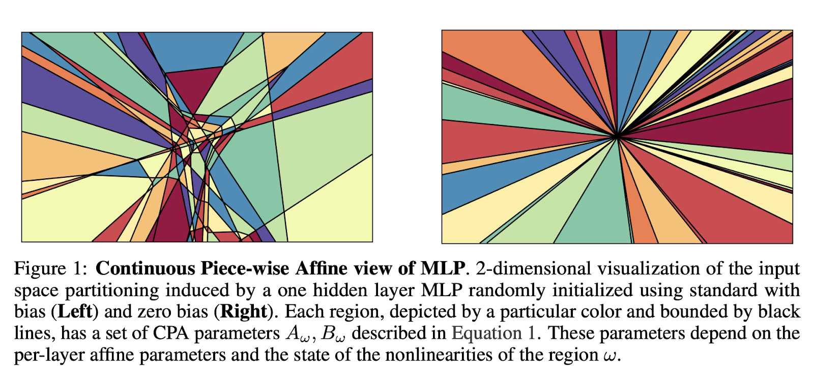
In modern neural architectures, we often remove bias terms for normalization purposes. Geometrically, this constrains our hyperplanes to pass through the origin. While this might seem limiting, it actually provides beneficial regularization properties and simplifies optimization. The figure above shows the geometric view of this choice.

Understanding LoRA

One interesting application of this geometric perspective comes in understanding low-rank adaptation methods like LoRA. This technique works by:

(W + AB)x: LoRA is a low-rank learning approach where one has an additive component, a product of two low rank (non-square, skinny or tall) matrices A and B. The idea allows for minimal fine-tuning or learning where one

• Focuses on efficiency through rank reduction
• Simple and effective for many tasks
• Does not explicitly prevent forgetting

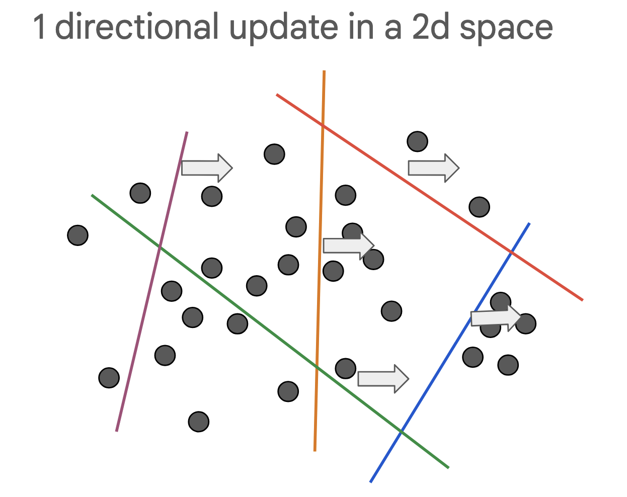
Geometrically, this is equivalent to

1. Updating the partitions only in a specific direction
2. Effective for tasks that are close to the pre-training distribution. Typically, LoRA does not result in new partitions as the hyperplane movements are severely constrained.
3. Note that the mapping in the partitions is changed, and thus, LoRA does not explicitly avoid forgetting.

Conclusion and Implications

Viewing MLPs as hashing functions provides a powerful mental model for understanding deep learning. By thinking about neural networks in terms of partitions and mappings, we can develop more intuitive approaches to architecture design, optimization, and adaptation.

This geometric perspective has several practical applications:

1. Better understanding of model capacity and memorization
2. More intuitive approaches to model compression
3. Improved techniques for adaptation and transfer learning

Moreover, this view of deep learning has led to interesting research directions in my own works, particularly in:

• Understanding and adapting transformer architectures (especially the interaction between attention and feed-forward layers)
• Developing better safety, constraint mechanisms
• Improving model reasoning capabilities